Commodity supply
Each area owns a certain percentage of the total global commodity volume produced (supplied). The global commodity supply side is modeled as one single sector, and its output is then divided among the individual areas using the commodity distribution parameters \(\lambda_t^{aa}\). Each area's demand for (use of) commodity can be lower or higher than its own share of global commodity supply; in that case, the area becomes a net commodity exporter or importer.
Global commodity extraction
$$ \newcommand{\tsum}{\textstyle\sum} \newcommand{\extern}[1]{\mathrm{\mathbf{{#1}}}} \newcommand{\local}{\mathrm{local}} \newcommand{\roc}[1]{\overset{\scriptsize\Delta}{#1{}}} \newcommand{\ss}{\mathrm{ss}} \newcommand{\aa}{\mathrm{aa}} \newcommand{\bb}{\mathrm{bb}} \newcommand{\E}{\mathrm{E}} \newcommand{\ref}{{\mathrm{ref}}} \newcommand{\blog}{\mathbf{log}\ } \newcommand{\bmax}{\mathbf{max}\ } \newcommand{\bDelta}{\mathbf{\Delta}} \newcommand{\bPi}{\mathbf{\Pi}} \newcommand{\bU}{\mathbf{U}} \newcommand{\newl}{\\[8pt]} \newcommand{\betak}{\mathit{zk}} \newcommand{\betay}{\mathit{zy}} \newcommand{\gg}{\mathrm{gg}} \newcommand{\tsum}{\textstyle{\sum}} \newcommand{\xnf}{\mathit{nf}} \newcommand{\ratio}[2]{\Bigl[\textstyle{\frac{#1}{#2}}\Bigr]} \newcommand{\unc}{\mathrm{unc}} \notag $$
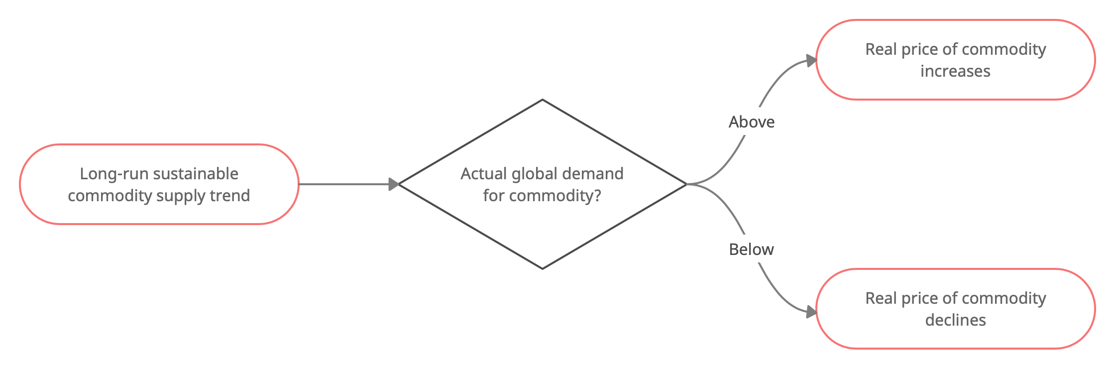
The total amount of commodities extracted globally, \(q_t^\gg\), follows a long-run supply trend, \(qq_t^\gg\), and responds to demand fluctuations; the gap between the actual amount (demand) and the long-run supply trend is referred to as global excess demand, \(q^\mathrm{exc}_t\).
Long-run sustainable supply trend
where
-
\(\kappa_1 \equiv \roc{a}{}_\ss^\gg \cdot \roc{nn}{}_\ss^\gg\)
-
\(\kappa_2\) is reverse engineered so that \(qq_\ss = q_\ss\) (global demand equals long-run supply trend)
Actual global demand
-
Actual commodity production is completey demand driven in the short run
-
Oil producers are able to satisfy short-term demand peak from inventories
Geographical distribution of global production (endowment)
Excess demand
- Excess demand is defined by the extent to which actual commodity production exceeds its long-run sustainable trend
Global commodity price relative to noncommodity export price
GEES Commodity extraction module
Declare quantities
!variables(:commodity)

    "Long-run level of commodity supply" gg_qq
    "Global commodity demand" gg_q
    "Global excess demand in commodity market" gg_qexc
    "Global price of commodities" gg_pq
    "Global real price of commodities" gg_pq_to_pxx
    "Autonomous markup in real price of commodities !! $\mathit{aut}^\gg_\mathit{pq}$" gg_aut_pq


!log-variables !all-but


!parameters(:commodity :dynamic)

    "Excess demand elasticity of commodity prices !! $\iota_1^\gg$" gg_iota_1
    "A/R Long-run trend in commodity supply !! $\rho_\mathit{qq}^\gg$" gg_rho_qq
    gg_rho_aut_pq, gg_ss_aut_pq


!shocks(:commodity)

    "Shock to long-run level in commodity supply" gg_shk_qq
    "Shock to price of commodities" gg_shk_pq
    gg_shk_aut_pq
Define equations
!equations(:commodity)

    "Long-run level of global commodity production"
    log(gg_qq) = ...
        + gg_rho_qq * log(gg_ss_roc_a * gg_ss_roc_nt * gg_qq{-1}) ...
        + (1 - gg_rho_qq) * log(gg_a * gg_nn * (&gg_q / &gg_a / &gg_nn)) ...
        + gg_shk_qq ...
    !! gg_qq = gg_q;


    "Log excess demand in commodity market"
    gg_qexc = gg_q / gg_qq ...
    !! gg_qexc = 1;


    "Commodity supply curve"
    gg_pq = gg_aut_pq * gg_pxx * gg_qexc^gg_iota_1 * exp(gg_shk_pq) ...
    !! gg_pq = gg_aut_pq * gg_pxx;


    "Autonomous markup in real commodity price"
    log(gg_aut_pq) = ...
        + gg_rho_aut_pq * log(gg_aut_pq{-1}) ...
        + (1 - gg_rho_aut_pq) * log(gg_ss_aut_pq) ...
        + gg_shk_aut_pq ...
    !! gg_aut_pq = gg_ss_aut_pq;


    "Global real prices of commodities"
    gg_pq_to_pxx = gg_pq / gg_pxx;